To demonstrate our theory has good predictive validity, we need to divide all possible states of the world into a set that is predicted by our theory, and a set that is not predicted by our theory. We can then collect data, and if the results are in line with our prediction (repeatedly, across replication studies), our theory gains verisimilitude – it seems to be related to the truth. We can never know the truth, but by corroborating theoretical predictions, we can hope to get closer to it.
The most common division of states of the world that are predicted and not prediction by a theory in null-hypothesis significance testing is the following: An effect of exactly zero is not predicted by a theory, and all other effects are taken to corroborate the theoretical prediction. Here, I want to explain why this is a very weak hypothesis test. In certain lines of research, it might even be a pretty trivial prediction. Luckily, it is quite easy to perform much stronger tests of hypotheses. I’ll also explain how to do so in practice.
Risky Predictions
Take a look at the three circles below. Each circle represents all possible outcomes of an empirical test of a theory. The blue line illustrates the state of the world that was observed. The line could have fallen anywhere on the circle. We performed a study and found one specific outcome. The black area in the circle represents the states of the world that will be interpreted as falsifying our prediction, whereas the white area is interpreted as the states in the world that will be interpreted as corroborating our prediction.

In the figure on the left, only a tiny fraction of states of the world will falsify our prediction. This represents a hypothesis test where only an infinitely small portion of all possible states of the world is not in line with the prediction. A common example is a two-sided null-hypothesis significance test, which forbids (and tries to reject) only the state of the world where the true effect size is exactly zero.
In the middle circle, 50% of all possible outcomes falsify the prediction, and 50% corroborates it. A common example is a one-sided null-hypothesis test. If you predict the mean is larger than zero, this prediction is falsified by all states of the world where the true effect is either equal to zero, or smaller than zero. This means that half of all possible states of the world can no longer be interpreted as corroborating your prediction. The blue line, or observed state of the world in the experiment, happens to fall in the white area for the middle circle, so we can still conclude the prediction is supported. However, our prediction was already slightly more risky than in the circle on the left representing a two-sided test.
In the scenario in the right circle, almost all possible outcomes are not in line with our prediction – only 5% of the circle is white. Again, the blue line, our observed outcome, falls in this white area, and our prediction is confirmed. However, now our prediction is confirmed in a very risky test. There were many ways in which we could be wrong – but we were right regardless.
Although our prediction is confirmed in all three scenarios above, philosophers of science such as Popper and Lakatos would be most impressed after your prediction has withstood the most severe test (i.e., in the scenario illustrated by the right circle). Our prediction was most specific: 95% of possible outcomes were judged as falsifying our prediction, and only 5% of possible outcomes would be interpreted as support for our theory. Despite this high hurdle, our prediction was corroborated. Compare this to the scenario on the left – almost any outcome would have supported our theory. That our prediction was confirmed in the scenario in the left circle is hardly surprising.
Systematic Noise
The scenario in the left, where only a very small part of all possible outcomes is seen as falsifying a prediction, is very similar to how people commonly use null-hypothesis significance tests. In a null-hypothesis significance test, any effect that is not zero is interpreted as support for a theory. Is this impressive? That depends on the possible states of the world. According to Meehl, there are many situations where null-hypothesis significance tests are performed, but the true difference is highly unlikely to be exactly zero. Meehl is especially worried about research where there is room for systematic noise, or the crud factor.
Systematic noise can only be excluded in an ideal experiment. In this ideal experiment, there is perfect random assignment to conditions, and only one single thing can cause a difference, such as in a randomized controlled trial. Perfection is notoriously hard to achieve in practice. In any close to perfect experiment, there can be tiny factors that, although not being the main goal of the experiment, lead to differences between the experimental and control condition. Participants in the experimental condition might read more words, answer more questions, need more time, have to think more deeply, or process more novel information. Any of these things could slightly move the true effect size away from zero – without being related to the independent variable the researchers aimed to manipulate. This is why Meehl calls it systematic noise, and not random noise: The difference is reliable, but not due to something you are theoretically interested in.
Many experiments are not even close to perfect and consequently have a lot of room for systematic noise. And then there are many studies where there isn’t even random assignment to conditions, but where data is correlational. As an example of correlational data, think about research examining differences between women and men. If we examine differences between men and women, the subjects in our study can not be randomly assigned to a condition. In such non-experimental studies, it is possible that ‘everything is correlated to everything’. For example, men are on average taller than women, and as a consequence it is more common for a man to be asked to pick an object of a high shelf in a supermarket, than vice versa. If we then ask men and women ‘how often do you help strangers’ this average difference in height has some tiny but systematic effect on their responses. In this specific case, systematic noise moves the mean difference from zero to a slightly higher value for men – but an unknown number of other sources of systematic noise are at play, and these interact, leading to an unknown final true population difference that is very unlikely to be exactly zero.
I think there are experiments that, for all practical purposes, are controlled enough to make a null-hypothesis a valid and realistic model to test against. However, I also think that these experiments are much more limited than the current widespread use of null-hypothesis testing. There are many experiments where a test against a null-hypothesis is performed, while the null-hypothesis is not reasonable to entertain, and we can not expect the difference to be exactly zero.
In those studies (e.g., as in the experiment examining gender differences above) it is much more impressive to have a theory that is able to predict how big an effect is (approximately). In other words, we should aim for theories that make point predictions, or a bit more reasonably, given that most sciences have a hard time predicting a single exact value, range predictions.
Range Predictions
Making more risky range predictions has some important benefits over the widespread use of null-hypothesis tests. These benefits mean that even if a null-hypothesis test is defensible, it would be preferable if you could test a range prediction.
Making a more risky prediction gives your theory higher verisimilitude. You will get more credit in darts when you correctly predict you will hit the bullseye, than when you correctly predict you will hit the board. Similarly, you get more credit for the predictive power of your theory when you correctly predict an effect will fall within 0.5 scale points of 8 on a 10 point scale, than when you predict the effect will be larger than the midpoint of the scale. A theory allows you to make predictions, and a good theory allows you to make precise predictions.
Range predictions allow you to design a study that can be falsified based on clear criteria. If you specify the bounds within which an effect should fall, any effect that is either smaller or larger will falsify the prediction. For a traditional null-hypothesis test, an effect of 0.0000001 will officially still fall in the possible states of the world that support the theory. However, it is practically impossible to falsify such tiny differences from zero, because doing so would require huge resources.
To increase the falsifiability of psychological research, the lower bound of the range prediction can be used as the smallest effect size of interest. Designing a study that has high power for this smallest effect size of interest (for example, a Cohen’s d of 0.1) will lead to an informative result. If the threshold for the smallest effect size of interest is really is so close to zero (e.g., 0.0000001) that a researcher does not have the resources to design a high powered study that could falsify this prediction. Specifying this range prediction is still, useful, because then it is clear to everyone that we do not have the resources to falsify that prediction.
Many of the criticisms on p-values in null-hypothesis tests disappear when p-values are calculated for range predictions. In a traditional hypothesis test with at least some systematic noise (meaning the true effect differs slightly from zero) all studies where the null is not exactly true will lead to a significant effect with a large enough sample size. This makes it a boring prediction, and we will end up stating there is a ‘significant’ difference for tiny irrelevant effects. I expect this problem will become more important now that it is easier to get access to Big Data.
However, we don’t want just any effect to become statistically significant – we want theoretically relevant effects to be significant, but not theoretically irrelevant effects. A range prediction achieves this. If we expect effects between 0.1 and 0.3, an effect of 0.05 might be statistically different from 0 in a huge sample, but it is not support for our prediction. To provide support for a range prediction your prediction needs to be accurate.
Testing Range Predictions in Practice
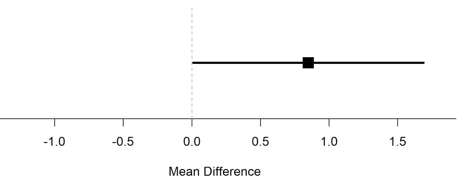
In a null-hypothesis test (visualized below) we compare the data against the hypothesis that the difference is 0 (indicated by the dotted vertical line at 0). The test yields a p = 0.047 – if we use an alpha level of 0.05, this is just below the alpha threshold. The observed difference (indicated by the square) has a confidence interval that ranges from almost 0 to 1.69. We can reject the null, but beyond that, we haven’t learned much.
In the example above, we were testing against a mean difference of 0. But there is no reason why a hypothesis test should be limited to test against a mean difference of 0. Meehl (1967 – yes, that is more than 40 years ago!) compared the use of statistical tests in psychology and physics, and notes that in physics, researchers make point predictions. For example, say a theory predicts a mean difference of 0.35. Let’s assume effects smaller than 0.1 are considered too small to matter, and effects larger than 0.6 are considered too large. Note that the bounds happen to be symmetric around the expected effect size (0.35 ±0.25) but you can set the bounds where ever you like. It is also perfectly acceptable not to specify an upper bound (in which case you are performing a minimal effects test, where you aim to reject effects smaller than a lower bound.
If you have learned about equivalence testing (see Lakens, Scheel, & Isager, 2018), you might recognize the practice of specifying equivalence bounds, and testing whether effects outside of this equivalence range can be rejected. In most equivalence tests the bounds are set up to fall on either size of 0 (e.g., -0.3 to 0.3), and the goal is to reject effect that are large enough to matter, so that we can conclude the effect is practically equivalent to zero.
But you can use equivalence tests to test any range. If you specify the bounds as ranging from 0.1 to 0.6, you can use for example the TOSTER package to test whether the observed effect is equivalent to the range of values you predicted. Below you see the hypothetical output for an experiment with n = 254 in two conditions, where ratings on a 7-point scale were collected from an experimental group (M = 5.25, SD = 1.12) and a control group (M = 4.87, SD = 0.98). A mean difference of 0.38 is observed, which is close to our predicted value of 0.35. We can set up an equivalence test to examine whether we can statistically conclude that we can reject effect sizes outside the range that we predicted. We can use the TOSTER package to test whether we can reject the presence of effects smaller than 0.1, and larger than 0.6. The code below performs the test for our range prediction:
library(TOSTER)
TOSTtwo.raw(m1 = 5.25,
m2 = 4.87,
sd1 = 1.12,
sd2 = 0.98,
n1 = 254,
n2 = 254,
low_eqbound = 0.1,
high_eqbound = 0.6,
alpha = 0.05,
var.equal = FALSE)
The results show we cannot just reject a mean difference of 0, we can also statistically reject values smaller than 0.1 and larger than 0.6:
Using alpha = 0.05 the equivalence test based on Welch's t-test was significant, t(497.2383) = -2.355984, p = 0.009430463
We have made a riskier prediction than a traditional two-sided hypothesis test, and our prediction was confirmed – impressive!

Note that although Meehl prefers point predictions that lie within a certain bound, he doesn’t completely reject the use of null-hypothesis significance testing. When he asks ‘Is it ever correct to use null-hypothesis significance tests?’ his own answer is ‘Of course it is’ (Meehl, 1990). There are times, such as very early in research lines, where researchers do not have good enough models, or reliable existing data, to make point predictions. Other times, two competing theories are not more precise than that one predicts rats in a maze will learn something, while the other theory predicts the rats will learn nothing. As Meehl writes: “When I was a rat psychologist, I unabashedly employed significance testing in latent-learning experiments; looking back I see no reason to fault myself for having done so in the light of my present methodological views.”
There are no good or bad statistical approaches – all statistical approaches are just answers to questions. What matters is asking the best possible question. It makes sense to allow traditional null-hypothesis tests early in research lines, when theories do not make more specific predictions than that ‘something’ will happen. But we should also push ourselves to develop theories that make more precise range predictions, and then test these more specific predictions. More mature theories should be able to predict effects in some range – even when these ranges are relatively wide.
The narrower the range you predict, the smaller the confidence interval needs to be to have a high probability of falling within the equivalence bounds (or to have high power for the equivalence test). Collecting a much larger sample size, with the direct real-world costs associated, might not immediately feel worth it, just for the lofty reward of higher verisimilitude (a concept philosophers don’t even know how to quantify!).
But thinking about hypothesis tests as range predictions is a useful skill. A two-sided null-hypothesis test sets the range of predictions to anywhere but zero. A one-sided test halves all possible states of the world that are predicted. This is a very efficient way to gain verisimilitude – indeed, because you can now only make Type 1 error in one direction, you even have the benefit of a small increase in power when performing a one-sided test. You could even go a step further, and instead of testing against the value of 0, acknowledge that there might be some systematic noise you are not interested in, and test against an effect of 0.05 (known as a minimal effects test). And finally, if you have a good theory, and see value in confirming a point prediction, you might want to put in the effort to collect enough data to test a range prediction (e.g., a difference between 0.3 and 0.6). All these tests use the same philosophical and statistical framework but make increasingly narrow range predictions. Thinking more carefully about the range of effects you want to corroborate or falsify, and relying less often on two-sided null-hypothesis tests, will make your hypothesis tests much stronger.
References
Lakens, D., Scheel, A. M., & Isager, P. M. (2018). Equivalence Testing for Psychological Research: A Tutorial. Advances in Methods and Practices in Psychological Science, 2515245918770963. https://doi.org/10/gdj7s9
Meehl, P. E. (1967). Theory-testing in psychology and physics: A methodological paradox. Philosophy of Science, 103–115.
Meehl, P. E. (1990). Appraising and amending theories: The strategy of Lakatosian defense and two principles that warrant it. Psychological Inquiry, 1(2), 108–141.