A preprint ("Justify Your Alpha: A Primer on Two Practical
Approaches") that extends and improves the ideas in this blog post is available at:
https://psyarxiv.com/ts4r6
Testing whether observed data should surprise us, under the assumption that some model of the data is true, is a widely used procedure in psychological science. Tests against a null model, or against the smallest effect size of interest for an equivalence test, can guide your decisions to continue or abandon research lines. Seeing whether a p-value is smaller than an alpha level is rarely the only thing you want to do, but especially early on in experimental research lines where you can randomly assign participants to conditions, it can be a useful thing.
Regrettably, this procedure is performed rather mindlessly. Doing Neyman-Pearson hypothesis testing well, you should carefully think about the error rates you find acceptable. How often do you want to miss the smallest effect size you care about, if it is really there? And how often do you want to say there is an effect, but actually be wrong? It is important to justify your error rates when designing an experiment. In this post I will provide one justification for setting the alpha level (something we recommended makes more sense than using a fixed alpha level).
Papers explaining how to justify your alpha level are very rare (for an example, see Mudge, Baker, Edge, & Houlahan, 2012). Here I want to discuss one of the least known, but easiest suggestions on how to justify alpha levels in the literature, proposed by Good. The idea is simple, and has been supported by many statisticians in the last 80 years: Lower the alpha level as a function of your sample size.
The idea behind this recommendation is most extensively discussed in a book by Leamer (1978, p. 92). He writes:
The rule of thumb quite popular now, that is, setting the significance level arbitrarily to .05, is shown to be deficient in the sense that from every reasonable viewpoint the significance level should be a decreasing function of sample size.
Leamer (you can download his book for free) correctly notes that this behavior, an alpha level that is a decreasing function of the sample size, makes sense from both a Bayesian as a Neyman-Pearson perspective. Let me explain.
Imagine a researcher who performs a study that has 99.9% power to detect the smallest effect size the researcher is interested in, based on a test with an alpha level of 0.05. Such a study also has 99.8% power when using an alpha level of 0.03. Feel free to follow along here, by setting the sample size to 204, the effect size to 0.5, alpha or p-value (upper limit) to 0.05, and the p-value (lower limit) to 0.03.
We see that if the alternative hypothesis is true only 0.1% of the observed studies will, in the long run, observe a p-value between 0.03 and 0.05. When the null-hypothesis is true 2% of the studies will, in the long run, observe a p-value between 0.03 and 0.05. Note how this makes p-values between 0.03 and 0.05 more likely when there is no true effect, than when there is an effect. This is known as Lindley’s paradox (and I explain this in more detail in Assignment 1 in my MOOC, which you can also do here).
Although you can argue that you are still making a Type 1 error at most 5% of the time in the above situation, I think it makes sense to acknowledge there is something weird about having a Type 1 error of 5% when you have a Type 2 error of 0.1% (again, see Mudge, Baker, Edge, & Houlahan, 2012, who suggest balancing error rates). To me, it makes sense to design a study where error rates are more balanced, and a significant effect is declared for p-values more likely to occur when the alternative model is true than when the null model is true.
Because power increases as the sample size increases, and because Lindley’s paradox (Lindley, 1957, see also Cousins, 2017) can be prevented by lowering the alpha level sufficiently, the idea to lower the significance level as a function of the sample is very reasonable. But how?
Zellner (1971) discusses how the critical value for a frequentist hypothesis test approaches a limit as the sample size increases (i.e., a critical value of 1.96 for p = 0.05 in a two-sided test) whereas the critical value for a Bayes factor increases as the sample size increases (see also Rouder, Speckman, Sun, Morey, & Iverson, 2009). This difference lies at the heart of Lindley’s paradox, and under certain assumptions comes down to a factor of √n. As Zellner (1971, footnote 19, page 304) writes (K01 is the formula for the Bayes factor):
If a sampling theorist were to adjust his significance level upward as n grows larger, which seems reasonable, za would grow with n and tend to counteract somewhat the influence of the √n factor in the expression for K01.
Jeffreys (1939) discusses Neyman and Pearson’s work and writes:
We should therefore get the best result, with any distribution of α, by some form that makes the ratio of the critical value to the standard error increase with n. It appears then that whatever the distribution may be, the use of a fixed P limit cannot be the one that will make the smallest number of mistakes.
He discusses the issue more in Appendix B, where he compared his own test (Bayes factors) against Neyman-Pearson decision procedures, and he notes that:
In spite of the difference in principle between my tests and those based on the P integrals, and the omission of the latter to give the increase of the critical values for large n, dictated essentially by the fact that in testing a small departure found from a large number of observations we are selecting a value out of a long range and should allow for selection, it appears that there is not much difference in the practical recommendations. Users of these tests speak of the 5 per cent. point in much the same way as I should speak of the K = 10-½ point, and of the 1 per cent. point as I should speak of the K = I0-1 point; and for moderate numbers of observations the points are not very different. At large numbers of observations there is a difference, since the tests based on the integral would sometimes assert significance at departures that would actually give K > I. Thus there may be opposite decisions in such cases. But they will be very rare.
So even though extremely different conclusions between Bayes factors and frequentist tests will be rare, according to Jeffreys, when the sample size grows, the difference becomes noticeable.
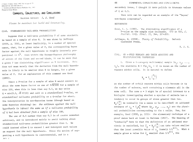
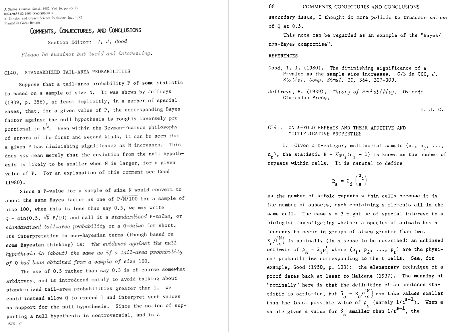
This brings us to Good’s (1982) easy solution. His paper is basically just a single page (I’d love something akin to a Comments, Conjectures, and Conclusions format in Meta-Psychology! – note that Good himself was the section editor, which started with ‘Please be succinct but lucid and interesting’, and it reads just like a blog post).
 He also explains the rationale in Good (1992):
‘we have empirical evidence that sensible P values are related to weights of evidence and, therefore, that P values are not entirely without merit. The real objection to P values is not that they usually are utter nonsense, but rather that they can be highly misleading, especially if the value of N is not also taken into account and is large.
Based on the observation by Jeffrey’s (1939) that, under specific circumstances, the Bayes factor against the null-hypothesis is approximately inversely proportional to √N, Good (1982) suggests a standardized p-value to bring p-values in closer relationship with weights of evidence:
Based on the observation by Jeffrey’s (1939) that, under specific circumstances, the Bayes factor against the null-hypothesis is approximately inversely proportional to √N, Good (1982) suggests a standardized p-value to bring p-values in closer relationship with weights of evidence:

Good doesn’t give a lot of examples of how standardized p-values should be used in practice, but I guess it makes things easier to think about a standardized alpha level (even though the logic is the same, just like you can double the p-value, or halve the alpha level, when you are correcting for 2 comparisons in a Bonferroni correction). So instead of an alpha level of 0.05, we can think of a standardized alpha level:

Again, with 100 participants α and αstan are the same, but as the sample size increases above 100, the alpha level becomes smaller. For example, a α = .05 observed in a sample size of 500 would have a αstan of 0.02236.
So one way to justify your alpha level is by using a decreasing alpha level as the sample size increases. I for one have always thought it was rather nonsensical to use an alpha level of 0.05 in all meta-analyses (especially when testing a meta-analytic effect size based on thousands of participants against zero), or large collaborative research project such as Many Labs, where analyses are performed on very large samples. If you have thousands of participants, you have extremely high power for most effect sizes original studies could have detected in a significance test. With such a low Type 2 error rate, why keep the Type 1 error rate fixed at 5%, which is so much larger than the Type 2 error rate in these analyses? It just doesn’t make any sense to me. Alpha levels in meta-analyses or large-scale data analyses should be lowered as a function of the sample size. In case you are wondering: an alpha level of .005 would be used when the sample size is 10.000.
When designing a study based on a specific smallest effect size of interest, where you desire to have decent power (e.g., 90%), we run in to a small challenge because in the power analysis we now have two unknowns: The sample size (which is a function of the power, effect size, and alpha), and the standardized alpha level (which is a function of the sample size). Luckily, this is nothing that some R-fu can’t solve by some iterative power calculations. [R code to calculate the standardized alpha level, and perform an iterative power analysis, is at the bottom of the post]
When we wrote Justify Your Alpha (I recommend downloading the original draft before peer review because it has more words and more interesting references) one of the criticism I heard the most is that we gave no solutions how to justify your alpha. I hope this post makes it clear that statisticians have discussed that the alpha level should not be any fixed value even since it was invented. There are already some solutions available in the literature. I like Good’s approach because it is simple. In my experience, people like simple solutions. It might not be a full-fledged decision theoretical cost-benefit analysis, but it beats using a fixed alpha level. I recently used it in a submission for a Registered Report. At the same time, I think it has never been used in practice, so I look forward to any comments, conjectures, and conclusions you might have.
Good, I. J. (1988). The interface between statistics and philosophy of science. Statistical Science, 3(4), 386–397.
Good, I. J. (1992). The Bayes/Non-Bayes Compromise: A Brief Review. Journal of the American Statistical Association, 87(419), 597. https://doi.org/10.2307/2290192
Lakens, D., Adolfi, F. G., Albers, C. J., Anvari, F., Apps, M. A. J., Argamon, S. E., … Zwaan, R. A. (2018). Justify your alpha. Nature Human Behaviour, 2, 168–171. https://doi.org/10.1038/s41562-018-0311-x
Leamer, E. E. (1978). Specification Searches: Ad Hoc Inference with Nonexperimental Data (1 edition). New York usw.: Wiley.
Mudge, J. F., Baker, L. F., Edge, C. B., & Houlahan, J. E. (2012). Setting an Optimal α That Minimizes Errors in Null Hypothesis Significance Tests. PLOS ONE, 7(2), e32734. https://doi.org/10.1371/journal.pone.0032734
Rouder, J. N., Speckman, P. L., Sun, D., Morey, R. D., & Iverson, G. (2009). Bayesian t tests for accepting and rejecting the null hypothesis. Psychonomic Bulletin & Review, 16(2), 225–237. https://doi.org/10.3758/PBR.16.2.225
Zellner, A. (1971). An introduction to Bayesian inference in econometrics. New York: Wiley.