A preprint ("Justify Your Alpha: A Primer on Two Practical Approaches") that extends the ideas in this blog post is available at: https://psyarxiv.com/ts4r6
In 1957 Neyman wrote: “it appears desirable to determine the level of significance in accordance with quite a few circumstances that vary from one particular problem to the next.” Despite this good advice, social scientists developed the norm to always use an alpha level of 0.05 as a threshold when making predictions. In this blog post I will explain how you can set the alpha level so that it minimizes the combined Type 1 and Type 2 error rates (thus efficiently making decisions), or balance Type 1 and Type 2 error rates. You can use this approach to justify your alpha level, and guide your thoughts about how to design studies more efficiently.
Neyman (1933) provides an example of the reasoning process he believed researchers should go through. He explains how a researcher might have derived an important hypothesis that H0 is true (there is no effect), and will not want to ‘throw it aside too lightly’. The researcher would choose a ow alpha level (e.g., 0.01). In another line of research, an experimenter might be interesting in detecting factors that would lead to the modification of a standard law, where the “importance of finding some new line of development here outweighs any loss due to a certain waste of effort in starting on a false trail”, and Neyman suggests to set the alpha level to for example 0.1.
Which is worse? A Type 1 Error or a Type 2 Error?
As you perform lines of research the data you collect are used as a guide to continue or abandon a hypothesis, to use one paradigm or another. One goal of well-designed experiments is to control the error rates as you make these decisions, so that you do not fool yourself too often in the long run.
Many researchers implicitly assume that Type 1 errors are more problematic than Type 2 errors. Cohen (1988) suggested a Type 2 error rate of 20%, and hence to aim for 80% power, but wrote “.20 is chosen with the idea that the general relative seriousness of these two kinds of errors is of the order of .20/.05, i.e., that Type I errors are of the order of four times as serious as Type II errors. This .80 desired power convention is offered with the hope that it will be ignored whenever an investigator can find a basis in his substantive concerns in his specific research investigation to choose a value ad hoc”. More recently, researchers have argued that false negative constitute a much more serious problem in science (Fiedler, Kutzner, & Krueger, 2012). I always ask my 3rd year bachelor students: What do you think? Is a Type 1 error in your next study worse than a Type 2 error?
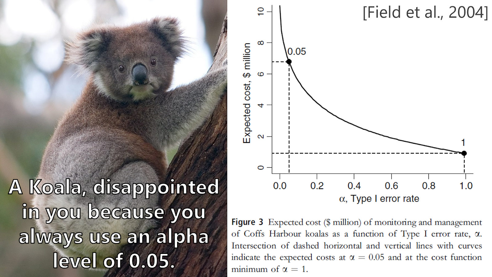
Last year I listened to someone who decided whether new therapies would be covered by the German healthcare system. She discussed Eye Movement Desensitization and Reprocessing (EMDR) therapy. I knew that the evidence that the therapy worked was very weak. As the talk started, I hoped they had decided not to cover EMDR. They did, and the researcher convinced me this was a good decision. She said that, although no strong enough evidence was available that it works, the costs of the therapy (which can be done behind a computer) are very low, it was applied in settings where no really good alternatives were available (e.g., inside prisons), and risk of negative consequences was basically zero. They were aware of the fact that there was a very high probability that EMDR was a Type 1 error, but compared to the cost of a Type 2 error, it was still better to accept the treatment. Another of my favorite examples comes from Field et al. (2004) who perform a cost-benefit analysis on whether to intervene when examining if a koala population is declining, and show the alpha should be set at 1 (one should always assume a decline is occurring and intervene).
Making these decisions is difficult - but it is better to think about them, then to end up with error rates that do not reflect the errors you actually want to make. As Ulrich and Miller (2019) describe, the long run error rates you actually make depend on several unknown factors, such as the true effect size, and the prior probability that the null hypothesis is true. Despite these unknowns, you can design studies that have good error rates for an effect size you are interested in, given some sample size you are planning to collect. Let's see how.
Balancing or minimizing error rates
Mudge, Baker, Edge, and Houlahan (2012) explain how researchers might want to minimize the total combined error rate. If both Type 1 as Type 2 errors are costly, then it makes sense to optimally reduce both errors as you do studies. This would make decision making overall most efficient. You choose an alpha level that, when used in the power analysis, leads to the lowest combined error rate. For example, with a 5% alpha and 80% power, the combined error rate is 5+20 = 25%, and if power is 99% and the alpha is 5% the combined error rate is 1 + 5 = 6%. Mudge and colleagues show that the increasing or reducing the alpha level can lower the combined error rate. This is one of the approaches we mentioned in our ‘Justify Your Alpha’ paper from 2018.
When we wrote ‘Justify Your Alpha’ we knew it would be a lot of work to actually develop methods that people can use. For months, I would occasionally revisit the code Mudge and colleagues used in their paper, which is an adaptation of the pwr library in R, but the code was too complex and I could not get to the bottom of how it worked. After leaving this aside for some months, during which I improved my R skills, some days ago I took a long shower and suddenly realized that I did not need to understand the code by Mudge and colleagues. Instead of getting their code to work, I could write my own code from scratch. Such realizations are my justification for taking showers that are longer than is environmentally friendly.
If you want to balance or minimize error rates, the tricky thing is that the alpha level you set determines the Type 1 error rate, but through it’s influence on the statistical power, also influenced the Type 2 error rate. So I wrote a function that examines the range of possible alpha levels (from 0 to 1) and minimizes either the total error (Type 1 + Type 2) or minimizes the difference between the Type 1 and Type 2 error rates, balancing the error rates. It then returns the alpha (Type 1 error rate) and the beta (Type 2 error). You can enter any analytic power function that normally works in R and would output the calculated power.
Minimizing Error Rates
Below is the version of the optimal_alpha function used in this blog. Yes, I am defining a function inside another function and this could all look a lot prettier - but it works for now. I plan to clean up the code when I archive my blog posts on how to justify alpha level in a journal, and will make an R package when I do.
The code requires requires you to specify the power function (in a way that the code returns the power, hence the $power at the end) for your test, where the significance level is a variable ‘x’. In this power function you specify the effect size (such as the smallest effect size you are interested in) and the sample size. In my experience, sometimes the sample size is determined by factors outside the control of the researcher. For example, you are working with a existing data, or you are studying a sample size that is limited (e.g., all students in a school). Other times, people have a maximum sample size they can feasibly collect, and accept the error rates that follow from this feasibility limitation. If your sample size is not limited, you can increase the sample size until you are happy with the error rates.
The code calculates the Type 2 error (1-power) across a range of alpha values. For example, we want to calculate the optimal alpha level for a independent t-test. Assume our smallest effect size of interest is d = 0.5, and we are planning to collect 100 participants in each group. We would normally calculate power as follows:
pwr.t.test(d = 0.5, n = 100, sig.level = 0.05, type = 'two.sample', alternative = 'two.sided')$power
This analysis tells us that we have 94% power with a 5% alpha level for our smallest effect size of interest, d = 0.5, when we collect 100 participants in each condition.
If we want to minimize our total error rates, we would enter this function in our optimal_alpha function (while replacing the sig.level argument with ‘x’ instead of 0.05, because we are varying the value to determine the lowest combined error rate).
res = optimal_alpha(power_function = pwr.t.test(d=0.5, n=100, sig.level = x, type='two.sample', alternative='two.sided')$power")
res$alpha
## [1] 0.05101728
res$beta
## [1] 0.05853977
We see that an alpha level of 0.051 slightly improved the combined error rate, since it will lead to a Type 2 error rate of 0.059 for a smallest effect size of interest of d = 0.5. The combined error rate is 0.11. For comparison, lowering the alpha level to 0.005 would lead to a much larger combined error rate of 0.25.
What would happen if we had decided to collect 200 participants per group, or only 50? With 200 participants per group we would have more than 99% power for d = 0.05, and relatively speaking, a 5% Type 1 error with a 1% Type 2 error is slightly out of balance. In the age of big data, we nevertheless researchers use such suboptimal error rates this all the time due to their mindless choice for an alpha level of 0.05. When power is large the combined error rates can be smaller if the alpha level is lowered. If we just replace 100 by 200 in the function above, we see the combined Type 1 and Type 2 error rate is the lowest if we set the alpha level to 0.00866. If you collect large amounts of data, you should really consider lowering your alpha level.
If the maximum sample size we were willing to collect was 50 per group, the optimal alpha level to reduce the combined Type 1 and Type 2 error rates is 0.13. This means that we would have a 13% probability of deciding there is an effect when the null hypothesis is true. This is quite high! However, if we had used a 5% Type 1 error rate, the power would have been 69.69%, with a 30.31% Type 2 error rate, while the Type 2 error rate is ‘only’ 16.56% after increasing the alpha level to 0.13. We increase the Type 1 error rate by 8%, to reduce the Type 2 error rate by 13.5%. This increases the overall efficiency of the decisions we make.
This example relies on the pwr.t.test function in R, but any power function can be used. For example, the code to minimize the combined error rates for the power analysis for an equivalence test would be:
res = optimal_alpha(power_function = "powerTOSTtwo(alpha=x, N=200, low_eqbound_d=-0.4, high_eqbound_d=0.4)")
Balancing Error Rates
You can choose to minimize the combined error rates, but you can also decide that it makes most sense to you to balance the error rates. For example, you think a Type 1 error is just as problematic as a Type 2 error, and therefore, you want to design a study that has balanced error rates for a smallest effect size of interest (e.g., a 5% Type 1 error rate and a 5% Type 2 error rate). Whether to minimize error rates or balance them can be specified in an additional argument in the function. The default it to minimize, but by adding error = "balance" an alpha level is given so that the Type 1 error rate equals the Type 2 error rate.
res = optimal_alpha(power_function = "pwr.t.test(d=0.5, n=100, sig.level = x, type='two.sample', alternative='two.sided')$power", error = "balance")
res$alpha
## [1] 0.05488516
res$beta
## [1] 0.05488402
Repeating our earlier example, the alpha level is 0.055, such that the Type 2 error rate, given the smallest effect size of interest and the and the sample size, is also 0.055. I feel that even though this does not minimize the overall error rates, it is a justification strategy for your alpha level that often makes sense. If both Type 1 and Type 2 errors are equally problematic, we design a study where we are just as likely to make either mistake, for the effect size we care about.
Relative costs and prior probabilities
So far we have assumed a Type 1 error and Type 2 error are equally problematic. But you might believe Cohen (1988) was right, and Type 1 errors are exactly 4 times as bad as Type 2 errors. Or you might think they are twice as problematic, or 10 times as problematic. However you weigh them, as explained by Mudge et al., 2012, and Ulrich & Miller, 2019, you should incorporate those weights into your decisions.
The function has another optional argument, costT1T2, that allows you to specify the relative cost of Type1:Type2 errors. By default this is set to 1, but you can set it to 4 (or any other value) such that Type 1 errors are 4 times as costly as Type 2 errors. This will change the weight of Type 1 errors compared to Type 2 errors, and thus also the choice of the best alpha level.
res = optimal_alpha(power_function = "pwr.t.test(d=0.5, n=100, sig.level = x, type='two.sample', alternative='two.sided')$power", error = "minimal", costT1T2 = 4)
res$alpha
## [1] 0.01918735
res$beta
## [1] 0.1211773
Now, the alpha level that minimized the weighted Type 1 and Type 2 error rates is 0.019.
Similarly, you can take into account prior probabilities that either the null is true (and you will observe a Type 1 error), or that the alternative hypothesis is true (and you will observe a Type 2 error). By incorporating these expectations, you can minimize or balance error rates in the long run (assuming your priors are correct). Priors can be specified using the prior_H1H0 argument, which by default is 1 (H1 and H0 are equally likely). Setting it to 4 means you think the alternative hypothesis (and hence, Type 2 errors) are 4 times more likely than that the null hypothesis (and Type 1 errors).
res = optimal_alpha(power_function = "pwr.t.test(d=0.5, n=100, sig.level = x, type='two.sample', alternative='two.sided')$power", error = "minimal", prior_H1H0 = 2)
res$alpha
## [1] 0.07901679
res$beta
## [1] 0.03875676
If you think H1 is four times more likely to be true than H0, you need to worry less about Type 1 errors, and now the alpha that minimizes the weighted error rates is 0.079. It is always difficult to decide upon priors (unless you are Omniscient Jones) but even if you ignore them, you are making the decision that H1 and H0 are equally plausible.
Conclusion
You can't abandon a practice without an alternative. Minimizing the combined error rate, or balancing error rates, provide two alternative approaches to the normative practice of setting the alpha level to 5%. Together with the approach to reduce the alpha level as a function of the sample size, I invite you to explore ways to set error rates based on something else than convention. A downside of abandoning mindless statistics is that you need to think of difficult questions. How much more negative is a Type 1 error than a Type 2 error? Do you have an ideas about the prior probabilities? And what is the smallest effect size of interest? Answering these questions is difficult, but considering them is important for any study you design. The experiments you make might very well be more informative, and more efficient. So give it a try.