In this blog, I'll explain how p-hacking will not lead to a peculiar prevalence of p-values just below .05 (e.g., in the 0.045-0.05 range) in the literature at large, but will instead lead to a difficult to identify increase in the Type 1 error rate across the 0.00-0.05 range. I re-analyze data by Masicampo & LaLande (2012), and try to provide a better model of the p-values they have observed through simulations in R (code below). I'd like to thank E.J. Masicampo and Daniel LaLande for sharing and allowing me to share their data, as well as their quick response to questions and a draft of this post. Thanks to Ryne Sherman for his p-hack code in R, to Nick Brown for asking me how M&L's article related to my previous blog post and for comments and suggestions on this post, and Tal Yarkoni for feedback on an earlier draft.
Masicampoand LaLande (2012; M&L) assessed the distribution of all 3627 p-values between 0.01 and 0.10 in 12
issues of the three journals. Exact p-values
were calculated from t-tests and F-tests. The authors conclude “The
number of p-values in the psychology
literature that barely meet the criterion for statistical significance (i.e.,
that fall just below .05) is unusually large”. “Specifically, the number of p-values between .045 and .050 was
higher than that predicted based on the overall distribution of p.”
There
are four factors that determine the distribution of p-values:
1) the number of
studies examining true effect and false effects
2) the power of
the studies that examine true effects
3) the frequency
of Type 1 error rates (and how they were inflated)
4) publication
bias.
Due
to publication bias, we should expect a substantial drop in the frequency with
which p-values above .05 appear in
the literature. True effects yield a right-skewed p-value distribution (the higher the power, the steeper the curve. e.g., Sellke, Bayarri, & Berger, 2001).
When the null-hypothesis is true the p-curve
is uniformly distributed, but when the Type 1 error rate is inflated due to
flexibility in the data-analysis, the p-value
distribution could become left-skewed below p-values
of .05.
M&L
model p-values based on a single
exponential curve estimation procedure that provides the best fit of p-values between .01 and .10. This is
not a valid approach because p-values
above and below p=.05 do not lie on a
continuous curve due to publication bias. It is therefore not surprising, nor
indicative of a prevalence of p-values
just below .05, that their single curve doesn’t fit the data very well, nor
that Chi-squared tests show the residuals (especially those just below .05) are
not randomly distributed.
P-hacking
does not create a peak in p-values just
below .05. Actually, p-hacking does
not even have to lead to a left-skewed p-value
distribution. If you perform multiple independent tests in a study, the p-value distribution is uniform, as if
you had performed 5 independent studies. The right skew emerges through
dependencies in the data in a repeated testing procedure. For example,
collecting data, performing a test, collecting additional data, and analyzing
the old and additional data together.
Figure
1 (left pane) shows p-value
distributions when H0 is true and researchers perform a test after 50 participants, and collect 10
additional participants for a maximum of 5 times, leading to a 15.4% Type 1
error rate, or (right pane) compare a single experimental condition to one of
five possible control conditions, leading to a Type 1 error rate of 18.2%. Only
5000 out of 100000 studies should yield a p<.05,
but we see an increase (above 500 for each of the 10 bins) across the range
from .00 to .05.

Identifying
a prevalence of Type 1 errors in a large heterogeneous set of studies is,
regrettably, even more problematic due to the p-value distribution of true effects. In Figure 2 (left) we see a p-distribution of 100000 experiments
with 50% power. Adding the 200000 experiments simulated above give the p-value
distribution on the right. Even when only 1/3rd of the studies
examines a true effect with a meager 51% power, it is already impossible to
observe a strong left-skewed distribution.

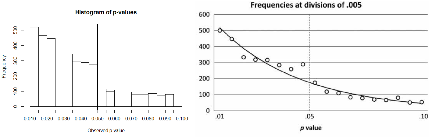
Do
frequencies of p-values just below p=.05 observed by M&L indicate
extreme p-hacking in a field almost
devoid of true effects? No. The striking illustration of the prevalence of p-values in Psychological Science just below .05 (Figure 3,
right, from M&L) from the blind rater is not apparent in the data coded by
the authors themselves (Figure 3, left, re-analysis based on the data kindly
provided by M&L). It is unclear what has led to the difference in coding by
the authors and the blind rater, but the frequencies between .03 and .05 look
like random variation due to the relatively small number of observations.

There
is also no evidence of a pre-valence of p-values
just below .05 when analyzing all p-values
collected by M&L. The authors find no peak when dividing the p-values in bins of .01, .005, or .0025,
and there is only a slight increase in the .04875-.05 range. There should be a
similar increase in the .0475-.04875 range, which is absent, and it is easier
to explain this pattern by random variation than by p-hacking.
As an example of a modeling approach of the p-value distribution based on power, Type 1 error rates and p-hacking, and publication bias, I’ve simulated 11000 studies with 41% power, taking into account publication bias by removing half of the studies with a p>.05, and added 4500 studies examining no real effect with an inflated Type 1 error rate of 18.2% (using the example above where an experimental study is compared to one of 5 control conditions). The R-script is available below. I do not mean to imply these parameters (the relative number of studies examining true vs. non true effects, power, the effect of publication bias, and the inflated Type 1 error rate) are typical for psychology, or even the most likely values for these parameters. I only mean to illustrate that choosing values for these four parameters is able to quite accurately simulate the p-value distribution actually observed by M&L. The true parameters require further empirical investigation. One interesting difference between my model and the observed p-values is a slight increase of p-values just above .05 – perhaps some leniency by reviewers to tend to accept studies with p-values that are almost statistically significant.
Even
though 839 of the 3877 simulated p-values
are Type 1 errors (614 of which are only significant through p-hacking) there is no noticeable
prevalence of p-values just below
.05. It is clear that p-hacking can
be a big problem even when it is difficult to observe. As such, the findings by
M&L clearly indicate publication bias (a large drop in p-values >.05), but do not necessarily identify a surprising
prevalence of p-values just below .05,
when interpreted against a more realistic model of expected p-value distributions. Concluding that p-hacking is a problem by analyzing a
large portion of the literature is practically impossible, unless there are a
huge amount of studies that use extreme flexibility in the data analysis.
An
alternative to attempting to point out p-hacking
in the entire psychological literature is to identify left-skewed p-curves in small sets of more
heterogeneous studies. Better yet, we should aim to control the Type 1 error
rate for the findings reported in an article. Pre-registration and/or replication (e.g., Nosek & Lakens, 2014)
are two approaches that can improve the reliability of findings.
You can download the data here (which E.J. Masicampo and Daniel LaLande gratiously allowed me to share). Store it at C:// and the code below will produce the left pane of Figure 3:
The R-code for the simulations in Figure 1 and 2 (Thanks to Ryne Sherman's p-hack script):
The R-code for the simulations in Figure 4:
References:
You can download the data here (which E.J. Masicampo and Daniel LaLande gratiously allowed me to share). Store it at C:// and the code below will produce the left pane of Figure 3:
library(foreign)
dataSPSS<-read.spss("C:/ML_QJEP2012_data.sav", to.data.frame=TRUE)
hist(dataSPSS$PS, xaxt="n", breaks=20, main="P-values in Psychological Science from M&L", xlab=("Observed p-value"))
axis(side = 1, at = c(0.01, 0.02, 0.03, 0.04, 0.05, 0.06, 0.07, 0.08, 0.09, 0.10))
abline(v=0.05, lwd=2)
The R-code for the simulations in Figure 1 and 2 (Thanks to Ryne Sherman's p-hack script):
The R-code for the simulations in Figure 4:
References:
Masicampo, E. J., & Lalande, D. R. (2012). A peculiar
prevalence of p-values just below. 05.
The Quarterly Journal of Experimental
Psychology, 65(11), 2271-2279.
Nosek, B. A.,
& Lakens, D. (2014). Registered reports: A method to increase the
credibility of published results. Social
Psychology, 43, 137-141. DOI:
10.1027/1864-9335/a000192.
Sellke, T., Bayarri, M. J., & Berger, J. O. (2001). Calibration
of p-values for testing precise null
hypotheses. The American Statistician,
55,62–71.
Big, big kudos to Masicampo and Lalande for /a/ sharing their data with you so readily, and /b/ allowing everyone else to see it. :-)
ReplyDeleteI couldn't agree more. This is now the third blog post in which I take a close look at results by other researchers, and every time people have been extremely helpful sharing data, insights, and comments. The scientific spirit is strong with this one!
DeleteThanks for this valuable post!
ReplyDeleteTwo discussion items:
1) I tried to repeat your simulations of Figure 1, right pane (in Matlab) and found that (logically) a steeper increase occurs across the range from 0 to 0.05 when not adding 10 participants each try, but when adding only 1 participant (e.g., as in Simmons, Nelson, & Simonsohn., 2011). Equivalently, increasing the sample size from 50 to 500 (but keeping 10 additions each try) also yields a sharp peak for p values just below 0.05. Trying more than 5 times also increases the peak of p-values just below 0.05. In other words, there might be p-hacking mechanisms which DO yield a preponderance of p-values just below 0.05.
2) Another way to identify p-hacking may be to look at longitudinal trends. For example, we found that p-values in the 0.041-0.049 range increased more steeply in the past 20 years than p-values in other ranges. I wonder what your opinion is on this… https://sites.google.com/site/jcfdewinter/DeRuiter_reply.pdf?attredirects=0
Kind regards
Hi Joost - yes, testing after every participant can really inflate the Type 1 error rate and create a peak. And if you assume 5000 studies do that, and only 1000 studies examine true effects, you can get a peak. But the observed data (by M&L and Kuhberger in my previous post) don't show such a peak just below .05. The question whether it is possible is less relevant than the question whether it happened.
DeleteAbout your paper: I have not looked at it carefully. If you want to do these analyses right, you should at least find a clear skewed p-value distribution, and only above this, and increase in a specific range over time, compared to other times. I don't know if your commentary is showing this - the ratio measure is very confusing. In absolute numbers, I think I see a p-curve that is as you'd expect. The ratio measure you focus on looks like it has a high risk of some artefact. But I'd have to look at it more carefully.
In sociology, p-values are almost always presented to two decimal places. Thus p = .05 covers the range .045 - .055. Yet we see in published articles that every instance of p = .05 is accompanied by an asterisk to denote p < .05! Roughly half of results where p (rounded to 2d.p.) = .05 are actually *not* statistically significant at the .05 level. This anomaly--which shows in a trivial way how much gamesmanship is involved in statistical analysis--should be easily proved by looking at a year's worth of articles in a top journal.
ReplyDeleteThe p-values were re-calculated from the test scores. People are not supposed to round a p-value of 0.054 down to p = .05 (but they do, see http://www.tandfonline.com/doi/abs/10.1080/17470218.2013.863371)
DeleteThanks for the reference to Leggett et al. 2013, it's a nice one!
DeleteI sat in my lounge room in Australia watching a documentary that was telling the story of a young Rohingya girl. https://www.fiverr.com/sabakhan695
ReplyDeleteThis comment has been removed by a blog administrator.
ReplyDeleteThis comment has been removed by a blog administrator.
ReplyDeleteThis comment has been removed by a blog administrator.
ReplyDeleteThis comment has been removed by a blog administrator.
ReplyDeleteThis comment has been removed by a blog administrator.
ReplyDelete