A blog on statistics, methods, philosophy of science, and open science. Understanding 20% of statistics will improve 80% of your inferences.

Showing posts with label NHST. Show all posts

Monday, September 20, 2021

Jerzy Neyman: A Positive Role Model in the History of Frequentist Statistics

Many of the facts in this blog post come from the biography ‘Neyman’ by Constance Reid. I highly recommend reading this book if you find this blog interesting.

In recent years researchers have become increasingly interested in the relationship between eugenics and statistics, especially focusing on the lives of Francis Galton, Karl Pearson, and Ronald Fisher. Some have gone as far as to argue for a causal relationship between eugenics and frequentist statistics. For example, in a recent book ‘Bernouilli’s Fallacy’, Aubrey Clayton speculates that Fisher’s decision to reject prior probabilities and embrace a frequentist approach was “also at least partly political”. Rejecting prior probabilities, Clayton argues, makes science seem more ‘objective’, which would have helped Ronald Fisher and his predecessors to establish eugenics as a scientific discipline, despite the often-racist conclusions eugenicists reached in their work.

When I was asked to review an early version of Clayton’s book for Columbia University Press, I thought that the main narrative was rather unconvincing, and thought the presented history of frequentist statistics was too one-sided and biased. Authors who link statistics to problematic political views often do not mention equally important figures in the history of frequentist statistics who were in all ways the opposite of Ronald Fisher. In this blog post, I want to briefly discuss the work and life of Jerzy Neyman, for two reasons.
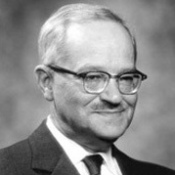

Jerzy Neyman (image from https://statistics.berkeley.edu/people/jerzy-neyman)

First, the focus on Fisher’s role in the history of frequentist statistics is surprising, given that the dominant approach to frequentist statistics used in many scientific disciplines is the Neyman-Pearson approach. If you have ever rejected a null hypothesis because a p-value was smaller than an alpha level, or if you have performed a power analysis, you have used the Neyman-Pearson approach to frequentist statistics, and not the Fisherian approach. Neyman and Fisher disagreed vehemently about their statistical philosophies (in 1961 Neyman published an article titled ‘Silver Jubilee of My Dispute with Fisher’), but it was Neyman’s philosophy that won out and became the default approach to hypothesis testing in most fields[i]. Anyone discussing the history of frequentist hypothesis testing should therefore seriously engage with the work of Jerzy Neyman and Egon Pearson. Their work was not in line with the views of Karl Pearson, Egon's father, nor the views of Fisher. Indeed, it was a great source of satisfaction to Neyman that their seminal 1933 paper was presented to the Royal Society by Karl Pearson, who was hostile and skeptical of the work, and (as Neyman thought) reviewed by Fisher[ii], who strongly disagreed with their philosophy of statistics.

Second, Jerzy Neyman was also the opposite to Fisher in his political viewpoints. Instead of promoting eugenics, Neyman worked to improve the position of those less privileged throughout his life, teaching disadvantaged people in Poland, and creating educational opportunities for Americans at UC Berkeley. He hired David Blackwell, who was the first Black tenured faculty member at UC Berkeley. This is important, because it falsifies the idea put forward by Clayton[iii] that frequentist statistics became the dominant approach in science because the most important scientists who worked on it wanted to pretend their dubious viewpoints were based on ‘objective’ scientific methods.  

I think it is useful to broaden the discussion of the history of statistics, beyond the work by Fisher and Karl Pearson, and credit the work of others[iv] who contributed in at least as important ways to the statistics we use today. I am continually surprised about how few people working outside of statistics even know the name of Jerzy Neyman, even though they regularly use his insights when testing hypotheses. In this blog, I will try to describe his work and life to add some balance to the history of statistics that most people seem to learn about. And more importantly, I hope Jerzy Neyman can be a positive role-model for young frequentist statisticians, who might so far have only been educated about the life of Ronald Fisher.


Neyman’s personal life


Neyman was born in 1894 in Russia, but raised in Poland. After attending the gymnasium, he studied at the University of Kharkov. Initially trying to become an experimental physicist, he was too clumsy with his hands, and switched to conceptual mathematics, in which he concluded his undergraduate in 1917 in politically tumultuous times. In 1919 he met his wife, and they marry in 1920. Ten days later, because of the war between Russia and Poland, Neyman is imprisoned for a short time, and in 1921 flees to a small village to avoid being arrested again, where he obtains food by teaching the children of farmers. He worked for the Agricultural Institute, and then worked at the University in Warsaw. He obtained his doctor’s degree in 1924 at age 30. In September 1925 he was sent to London for a year to learn about the latest developments in statistics from Karl Pearson himself. It is here that he met Egon Pearson, Karl’s son, and a friendship and scientific collaboration starts.

Neyman always spends a lot of time teaching, often at the expense of doing scientific work. He was involved in equal opportunity education in 1918 in Poland, teaching in dimly lit classrooms where the rag he used to wipe the blackboard would sometimes freeze. He always had a weak spot for intellectuals from ‘disadvantaged’ backgrounds. He and his wife were themselves very poor until he moved to UC Berkeley in 1938. In 1929, back in Poland, his wife becomes ill due to their bad living conditions, and the doctor who comes to examine her is so struck by their miserable living conditions he offers the couple stay in his house for the same rent they were paying while he visits France for 6 months. In his letters to Egon Pearson from this time, he often complained that the struggle for existence takes all his time and energy, and that he can not do any scientific work.

Even much later in his life, in 1978, he kept in mind that many people have very little money, and he calls ahead to restaurants to make sure a dinner before a seminar would not cost too much for the students. It is perhaps no surprise that most of his students (and he had many) talk about Neyman with a lot of appreciation. He wasn’t perfect (for example, Erich Lehmann - one of Neyman's students - remarks how he was no longer allowed to teach a class after Lehmann's notes, building on but extending the work by Neyman, became extremely popular – suggesting Neyman was no stranger to envy). But his students were extremely positive about the atmosphere he created in his lab. For example, job applicants were told around 1947 that “there is no discrimination on the basis of age, sex, or race ... authors of joint papers are always listed alphabetically."

Neyman himself often suffered discrimination, sometimes because of his difficulty mastering the English language, sometimes for being Polish (when in Paris a piece of clothing, and ermine wrap, is stolen from their room, the police responds “What can you expect – only Poles live there!”), sometimes because he did not believe in God, and sometimes because his wife was Russian and very emancipated (living independently in Paris as an artist). He was fiercely against discrimination. In 1933, as anti-Semitism is on the rise among students at the university where he works in Poland, he complains to Egon Pearson in a letter that the students are behaving with Jews as Americans do with people of color. In 1941 at UC Berkeley he hired women at a time it was not easy for a woman to get a job in mathematics.  

In 1942, Neyman examined the possibility of hiring David Blackwell, a Black statistician, then still a student. Neyman met him in New York (so that Blackwell does not need to travel to Berkeley at his own expense) and considered Blackwell the best candidate for the job. The wife of a mathematics professor (who was born in the south of the US) learned about the possibility that a Black statistician might be hired, warns she will not invite a Black man to her house, and there was enough concern for the effect the hire would have on the department that Neyman can not make an offer to Blackwell. He is able to get Blackwell to Berkeley in 1953 as a visiting professor, and offers him a tenured job in 1954, making David Blackwell the first tenured faculty member at the University of Berkeley, California. And Neyman did this, even though Blackwell was a Bayesian[v] ;).

In 1963, Neyman travelled to the south of the US and for the first time directly experienced the segregation. Back in Berkeley, a letter is written with a request for contributions for the Southern Christian Leadership Conference (founded by Martin Luther King, Jr. and others), and 4000 copies are printed and shared with colleagues at the university and friends around the country, which brought in more than $3000. He wrote a letter to his friend Harald Cramér that he believed Martin Luther King, Jr. deserved a Nobel Peace Prize (which Cramér forwarded to the chairman of the Nobel Committee, and which he believed might have contributed at least a tiny bit to fact that Martin Luther King, Jr. was awarded the Nobel Prize a year later). Neyman also worked towards the establishment of a Special Scholarships Committee at UC Berkeley with the goal of providing education opportunities to disadvantaged Americans

Neyman was not a pacifist. In the second world war he actively looked for ways he could contribute to the war effort. He is involved in statistical models that compute the optimal spacing of bombs by planes to clear a path across a beach of land mines. (When at a certain moment he needs specifics about the beach, a representative from the military who is not allowed to directly provide this information asks if Neyman has ever been to the seashore in France, to which Neyman replies he has been to Normandy, and the representative answers “Then use that beach!”). But Neyman early and actively opposed the Vietnam war, despite the risk of losing lucrative contracts the Statistical Laboratory had with the Department of Defense. In 1964 he joined a group of people who bought advertisements in local newspapers with a picture of a napalmed Vietnamese child with the quote “The American people will bluntly and plainly call it murder”.


A positive role model


It is important to know the history of a scientific discipline. Histories are complex, and we should resist overly simplistic narratives. If your teacher explains frequentist statistics to you, it is good if they highlight that someone like Fisher had questionable ideas about eugenics. But the early developments in frequentist statistics involved many researchers beyond Fisher[vi], and, luckily, there are many more positive role-models that also deserve to be mentioned - such as Jerzy Neyman. Even though Neyman’s philosophy on statistical inferences forms the basis of how many scientists nowadays test hypotheses, his contributions and personal life are still often not discussed in histories of statistics - an oversight I hope the current blog post can somewhat mitigate. If you want to learn more about the history of statistics through Neyman’s personal life, I highly recommend the biography of Neyman by Constance Reid, which was the source for most of the content of this blog post.


[i] See Hacking, 1965: “The mature theory of Neyman and Pearson is very nearly the received theory on testing statistical hypotheses.”

[ii] It turns out, in the biography, that it was not Fisher, but A. C. Aitken, who reviewed the paper positively.

[iii] Clayton’s book seems to be mainly intended as an attempt to persuade readers to become a Bayesian, and not as an accurate analysis of the development of frequentist statistics.

[iv] William Gosset (or 'Student', from 'Student's t-test'), who was the main inspiration for the work by Neyman and Pearson, is another giant in frequentist statistics who does not in any way fit into the narrative that frequentist statistics is tied to eugenics, as his statistical work was motivated by applied research questions in the Guinness brewery. Gosset was a modest man – which is probably why he rarely receives the credit he is due.

[v] When asked about his attitude towards Bayesian statistics in 1979, he answered: “It does not interest me. I am interested in frequencies.” He did note multiple legitimate approaches to statistics exist, and the choice one makes is largely a matter of personal taste. Neyman opposed subjective Bayesian statistics because their use could lead to bad decision procedures, but was very positive about later work by Wald, which inspired Bayesian statistical decision theory.

[vi] For a more nuanced summary of Fisher's life, see https://www.nature.com/articles/s41437-020-00394-6 


Thursday, March 12, 2020

What’s a family in family-wise error control?

When you perform multiple comparisons in a study, you need to control your alpha level for multiple comparisons. It is generally recommended to control for the family-wise error rate, but there is some confusion about what a 'family' is. As Bretz, Hothorn, & Westfall (2011) write in their excellent book “Multiple Comparisons Using R” on page 15: “The appropriate choice of null hypotheses being of primary interest is a controversial question. That is, it is not always clear which set of hypotheses should constitute the family H1,…,Hm. This topic has often been in dispute and there is no general consensus.” In one of the best papers on controlling for multiple comparisons out there, Bender & Lange (2001) write: “Unfortunately, there is no simple and unique answer to when it is appropriate to control which error rate. Different persons may have different but nevertheless reasonable opinions. In addition to the problem of deciding which error rate should be under control, it has to be defined first which tests of a study belong to one experiment.” The Wikipedia page on family-wise error rate is a mess.

I will be honest: I have never understood this confusion about what a family of tests is when controlling the family-wise error rate. At least not in a Neyman-Pearson approach to hypothesis testing, where the goal is to use data to make decisions about how to act. Neyman (Neyman, 1957) calls his approach inductive behavior. The outcome of an experiment leads one to take different possible actions, which can be either practical (e.g., implement a new procedure, abandon a research line) or scientific (e.g., claim there is or is no effect). From an error-statistical approach (Mayo, 2018) inflated Type 1 error rates mean that it has become very likely that you will be able to claim support for your hypothesis, even when the hypothesis is wrong. This reduces the severity of the test. To prevent this, we need to control our error rate at the level of our claim.

One reason the issue of family-wise error rates might remain vague, is that researchers are often vague about their claims. We do not specify our hypotheses unambiguously, and therefore this issue remains unclear. To be honest, I suspect another reason there is a continuing debate about whether and how to lower the alpha level to control for multiple comparisons in some disciplines is that 1) there are a surprisingly large number of papers written on this topic that argue you do not need to control for multiple comparisons, which are 2) cited a huge number of times giving rise to the feeling that surely they must have a point. Regrettably, the main reason these papers are written is because there are people who don't think a Neyman-Pearson approach to hypothesis testing is a good idea, and the main reason these papers are cited is because doing so is convenient for researchers who want to publish statistically significant results, as they can justify why they are not lowering their alpha level, making that p = 0.02 in one of three tests really 'significant'. All papers that argue against the need to control for multiple comparisons when testing hypotheses are wrong.  Yes, their existence and massive citation counts frustrate me. It is fine not to test a hypothesis, but when you do, and you make a claim based on a test, you need to control your error rates. 

But let’s get back to our first problem, which we can solve by making the claims people need to control Type 1 error rates for less vague. Lisa DeBruine and I recently proposed machine readable hypothesis tests to remove any ambiguity in the tests we will perform to examine statistical predictions, and when we will consider a claim corroborated or falsified. In this post, I am going to use our R package ‘scienceverse’ to clarify what constitutes a family of tests when controlling the family-wise error rate.

An example of formalizing family-wise error control


Let’s assume we collect data from 100 participants in a control and treatment condition. We collect 3 dependent variables (dv1, dv2, and dv3). In the population there is no difference between groups on any of these three variables (the true effect size is 0). We will analyze the three dv’s in independent t-tests. This requires specifying our alpha level, and thus deciding whether we need to correct for multiple comparisons. How we control error rates depends on claim we want to make.

We might want to act as if (or claim that) our treatment works if there is a difference between the treatment and control conditions on any of the three variables. In scienceverse terms, this means we consider the prediction corroborated when the p-value of the first t-test is smaller than alpha level, the p-value of the second t-test is smaller than the alpha level, or the p-value of the first t-test is smaller than the alpha level. In the scienceverse code, we specify a criterion for each test (a p-value smaller than the alpha level, p.value < alpha_level) and conclude the hypothesis is corroborated if either of these criteria are met ("p_t_1 | p_t_2 | p_t_3").  

We could also want to make three different predictions. Instead of one hypothesis (“something will happen”) we have three different hypotheses, and predict there will be an effect on dv1, dv2, and dv3. The criterion for each t-test is the same, but we now have three hypotheses to evaluate (H1, H2, and H3). Each of these claims can be corroborated, or not.

Scienceverse allows you to specify your hypotheses tests unambiguously (for code used in this blog, see the bottom of the post). It also allows you to simulate a dataset, which we can use to examine Type 1 errors by simulating data where no true effects exist. Finally, scienceverse allows you to run the pre-specified analyses on the (simulated) data, and will automatically create a report that summarizes which hypotheses were corroborated (which is useful when checking if the conclusions in a manuscript indeed follow from the preregistered analyses, or not). The output a single simulated dataset for the scenario where we will interpret any effect on the three dv’s as support for the hypothesis looks like this:

Evaluation of Statistical Hypotheses

12 March, 2020

Simulating Null Effects Postregistration

Results

Hypothesis 1: H1

Something will happen
  • p_t_1 is confirmed if analysis ttest_1 yields p.value<0.05

    The result was p.value = 0.452 (FALSE)

  • p_t_2 is confirmed if analysis ttest_2 yields p.value<0.05

    The result was p.value = 0.21 (FALSE)

  • p_t_3 is confirmed if analysis ttest_3 yields p.value<0.05

    The result was p.value = 0.02 (TRUE)

Corroboration ( TRUE )

The hypothesis is corroborated if anything is significant.
 p_t_1 | p_t_2 | p_t_3 

Falsification ( FALSE )

The hypothesis is falsified if nothing is significant.
 !p_t_1 & !p_t_2 & !p_t_3 
All criteria were met for corroboration.


We see the hypothesis that ‘something will happen’ is corroborated, because there was a significant difference on dv3 - even though this was a Type 1 error, since we simulated data with a true effect size of 0 - and any difference was taken as support for the prediction. With a 5% alpha level, we will observe 1-(1-0.05)^3 = 14.26% Type 1 errors in the long run. This Type 1 error inflation can be prevented by lowering the alpha level, for example by a Bonferroni correction (0.05/3), after which the expected Type 1 error rate is 4.92% (see Bretz et al., 2011, for more advanced techniques to control error rates). When we examine the report for the second scenario, where each dv tests a unique hypothesis, we get the following output from scienceverse:


Evaluation of Statistical Hypotheses

12 March, 2020

Simulating Null Effects Postregistration

Results

Hypothesis 1: H1

dv1 will show an effect
  • p_t_1 is confirmed if analysis ttest_1 yields p.value<0.05

    The result was p.value = 0.452 (FALSE)

Corroboration ( FALSE )

The hypothesis is corroborated if dv1 is significant.
 p_t_1 

Falsification ( TRUE )

The hypothesis is falsified if dv1 is not significant.
 !p_t_1 
All criteria were met for falsification.

Hypothesis 2: H2

dv2 will show an effect
  • p_t_2 is confirmed if analysis ttest_2 yields p.value<0.05

    The result was p.value = 0.21 (FALSE)

Corroboration ( FALSE )

The hypothesis is corroborated if dv2 is significant.
 p_t_2 

Falsification ( TRUE )

The hypothesis is falsified if dv2 is not significant.
 !p_t_2 
All criteria were met for falsification.

Hypothesis 3: H3

dv3 will show an effect
  • p_t_3 is confirmed if analysis ttest_3 yields p.value<0.05

    The result was p.value = 0.02 (TRUE)

Corroboration ( TRUE )

The hypothesis is corroborated if dv3 is significant.
 p_t_3 

Falsification ( FALSE )

The hypothesis is falsified if dv3 is not significant.
 !p_t_3 
All criteria were met for corroboration.


We now see that two hypotheses were falsified (yes, yes, I know you should not use p > 0.05 to falsify a prediction in real life, and this part of the example is formally wrong so I don't also have to explain equivalence testing to readers not familiar with it - if that is you, read this, and know scienceverse will allow you to specify equivalence test as the criterion to falsify a prediction, see the example here). The third hypothesis is corroborated, even though, as above, this is a Type 1 error.

It might seem that the second approach, specifying each dv as it’s own hypothesis, is the way to go if you do not want to lower the alpha level to control for multiple comparisons. But take a look at the report of the study you have performed. You have made 3 predictions, of which 1 was corroborated. That is not an impressive success rate. Sure, mixed results happen, and you should interpret results not just based on the p-value (but on the strength of the experimental design, assumptions about power, your prior, the strength of the theory, etc.) but if these predictions were derived from the same theory, this set of results is not particularly impressive. Since researchers can never selectively report only those results that ‘work’ because this would be a violation of the code of research integrity, we should always be able to see the meager track record of predictions.If you don't feel ready to make a specific predictions (and run the risk of sullying your track record) either do unplanned exploratory tests, and do not make claims based on their results, or preregister all possible tests you can think of, and massively lower your alpha level to control error rates (for example, genome-wide association studies sometimes use an alpha level of 5 x 10⁻⁸ to control the Type 1 erorr rate).

Hopefully, specifying our hypotheses (and what would corroborate them) transparently by using scienceverse makes it clear what happens in the long run in both scenarios. In the long run, both the first scenario, if we would use an alpha level of 0.05/3 instead of 0.05, and the second scenario, with an alpha level of 0.05 for each individual hypothesis, will lead to the same end result: Not more than 5% of our claims will be wrong, if the null hypothesis is true. In the first scenario, we are making one claim in an experiment, and in the second we make three. In the second scenario we will end up with more false claims in an absolute sense, but the relative number of false claims is the same in both scenarios. And that’s exactly the goal of family-wise error control.

References
Bender, R., & Lange, S. (2001). Adjusting for multiple testing—When and how? Journal of Clinical Epidemiology, 54(4), 343–349.
Bretz, F., Hothorn, T., & Westfall, P. H. (2011). Multiple comparisons using R. CRC Press.
Mayo, D. G. (2018). Statistical inference as severe testing: How to get beyond the statistics wars. Cambridge University Press.
Neyman, J. (1957). “Inductive Behavior” as a Basic Concept of Philosophy of Science. Revue de l’Institut International de Statistique / Review of the International Statistical Institute, 25(1/3), 7. https://doi.org/10.2307/1401671

Thanks to Lisa DeBruine for feedback on an earlier draft of this blog post.


Sunday, November 24, 2019

Do You Really Want to Test a Hypothesis?


I’ve uploaded one of my favorite lectures in the my new MOOC “Improving Your Statistical Questions” to YouTube. It asks the question whether you really want to test a hypothesis. A hypothesis is a very specific tool to answer a very specific question. I like hypothesis tests, because in experimental psychology it is common to perform lines of research where you can design a bunch of studies that test simple predictions about the presence or absence of differences on some measure. I think they have a role to play in science. I also think hypothesis testing is widely overused. As we are starting to do hypothesis tests better (e.g., by preregistering our predictions and controlling our error rates in more severe tests) I predict many people will start to feel a bit squeamish as they become aware that doing hypothesis tests as they were originally designed to be used isn’t really want they want in their research. One of the often overlooked gains in teaching people how to do something well, is that they finally realize that they actually don’t want to do it.

The lecture “Do You Really Want to Test a Hypothesis” aims to explain which question a hypothesis tests asks, and discusses when a hypothesis tests answers a question you are interested in. It is very easy to say what not to do, or to point out what is wrong with statistical tools. Statistical tools are very limited, even under ideal circumstances. It’s more difficult to say what you can do. If you follow my work, you know that this latter question is what I spend my time on. Instead of telling you optional stopping can’t be done because it is p-hacking, I explain how you can do it correctly through sequential analysis. Instead of telling you it is wrong to conclude the absence of an effect from p > 0.05, I explain how to use equivalence testing­­. Instead of telling you p-values are the devil, I explain how they answer a question you might be interested in when used well. Instead of saying preregistration is redundant, I explain from which philosophy of science preregistration has value. And instead of saying we should abandon hypothesis tests, I try to explain in this video how to use them wisely. This is all part of my ongoing #JustifyEverything educational tour. I think it is a reasonable expectation that researchers should be able to answer at least a simple ‘why’ question if you ask why they use a specific tool, or use a tool in a specific manner.

This might help to move beyond the simplistic discussion I often see about these topics. If you ask me if I prefer frequentist of Bayesian statistics, or confirmatory or exploratory research, I am most likely to respond 無 (see Wikipedia). It is tempting to think about these topics in a polarized either-or mindset – but then you would miss asking the real questions. When would any approach give you meaningful insights? Just as not every hypothesis test is an answer to a meaningful question, so will not every exploratory study provide interesting insights. The most important question to ask yourself when you plan a study is ‘when will the tools you use lead to interesting insights’? In the second week of my MOOC I discuss when effects in hypothesis tests could be deemed meaningful, but the same question applies to exploratory or descriptive research. Not all exploration is interesting, and we don’t want to simply describe every property of the world. Again, it is easy to dismiss any approach to knowledge generation, but it is so much more interesting to think about which tools will lead to interesting insights. And above all, realize that in most research lines, researchers will have a diverse set of questions that they want to answer given practical limitations, and they will need to rely on a diverse set of tools, limitations and all.

In this lecture I try to explain what the three limitations are of hypothesis tests, and the very specific question they try to answer. If you like to think about how to improve your statistical questions, you might be interested in enrolling in my free MOOC “Improving Your Statistical Questions”.